From the Navier–Stokes Equations to Aerodynamic Lift

Aerodynamic lift is often introduced with a simple statement: air moves faster over the upper surface of a wing, so the pressure there is lower, producing an upward force. While this statement contains part of the story, it hides most of the interesting physics.

A more satisfying way to understand lift is to start from the fundamental equations governing fluids, see why the general problem is difficult, and then progressively simplify the problem until we reach a special class of flows that can be solved analytically. The classical theory of Joukowski airfoils provides an especially beautiful example: a complicated three-dimensional viscous flow around a wing can be approximated, under suitable idealizations, by a two-dimensional potential-flow problem that can be solved using complex analysis and conformal mappings.

The resulting theory also reveals something important about lift: circulation is not merely a mathematical trick. It is the quantity that connects the flow around an airfoil to the lift force.

1. The fundamental equations of fluid dynamics

   A fluid is described by fields such as density, velocity, pressure, and temperature:

   $\rho \left(\overrightarrow{\mathbf{x}},t\right)$, $\overrightarrow{\mathbf{v}}\left(\overrightarrow{\mathbf{x}},t\right)$, $p\left(\overrightarrow{\mathbf{x}},t\right)$, $T\left(\overrightarrow{\mathbf{x}},t\right)$

   These fields are constrained by conservation laws (presented below in Eulerian form).

   The first is conservation of mass:

   $\frac{\partial \rho }{\partial t}+\overrightarrow{\mathbf{v}}\cdot \nabla \rho =-\rho \nabla \cdot \overrightarrow{\mathbf{v}}$

   The second is conservation of momentum. In continuum mechanics, this is expressed by the Cauchy momentum equation. For a simple fluid, decomposing the total stress into an isotropic pressure part and a viscous part gives:

   $\rho [\frac{\partial \overrightarrow{\mathbf{v}}}{\partial t}+(\overrightarrow{\mathbf{v}}\cdot \nabla \left)\overrightarrow{\mathbf{v}}\right]=-\nabla p+\nabla \cdot \mathbf{\tau }+\rho \overrightarrow{g}$

   where $\mathbf{\tau }$ is the viscous stress tensor. The total Cauchy stress tensor is therefore: $\mathbf{\sigma }=-p\mathbf{𝕀}+\mathbf{\tau }$

   The Cauchy equation itself does not yet specify how a particular fluid behaves. A constitutive relation for the stress tensor is required. For a Newtonian fluid, the viscous stress is related to the velocity gradients, and the momentum equation becomes the Navier–Stokes equation.

   Finally, conservation of energy gives an additional equation involving internal energy, mechanical work, heat conduction, and other forms of energy transfer. Here $e$ is the specific internal energy and $k$ is the thermal conductivity:

   $\rho [\frac{\partial }{\partial t}(e+\frac{{\left|\overrightarrow{\mathbf{v}}\right|}^2}{2})+\overrightarrow{\mathbf{v}}\cdot \nabla (e+\frac{{\left|\overrightarrow{\mathbf{v}}\right|}^2}{2})]=-\nabla \cdot (p\overrightarrow{\mathbf{v}})+\nabla \cdot \left(\mathbf{\tau }\overrightarrow{\mathbf{v}}\right)+\nabla \cdot (k\nabla T)+\rho \overrightarrow{\mathbf{g}}\cdot \overrightarrow{\mathbf{v}}$

   Thus the familiar equations of fluid dynamics are ultimately consequences of conservation laws together with constitutive assumptions about the material.

   For aerodynamic problems, one might therefore begin with the full compressible Navier–Stokes equations, the continuity equation, and the energy equation, together with an equation of state and appropriate constitutive relations.

   There is, however, an immediate problem.

   Knowing the equations does not mean that we can solve them.

2. Why calculating the lift of a real wing is difficult

   Suppose we know the exact shape of an aircraft wing and the velocity, pressure, temperature, and density of the air far away from it.

   In principle, we could solve the fluid equations and obtain the pressure and viscous stresses everywhere around the wing. The aerodynamic force would then follow from integrating the stress over the surface:

   $\overrightarrow{\mathbf{F}}=\underset{S}{∯}\mathbf{\sigma }\cdot d\overrightarrow{\mathbf{S}}$

   The lift is simply the component of this force perpendicular to the freestream direction.

   The difficulty is that the resulting system of coupled partial differential equations is nonlinear, primarily because of the convective term:

   $(\overrightarrow{\mathbf{v}}\cdot \nabla )\overrightarrow{\mathbf{v}}$

   Furthermore, the fluid must satisfy boundary conditions on the complicated surface of the wing, while the flow may contain boundary layers, separation, turbulence, wakes, vortices, and possibly compressibility effects.

   Consequently, even though the governing equations themselves are conceptually straightforward, obtaining an exact analytical solution for a realistic aircraft is generally not feasible.

   This motivates a central idea in theoretical aerodynamics:

   Instead of solving the complete problem, identify a simpler physical regime in which the dominant features of the phenomenon can still be understood.

   For lift, one particularly successful simplification is potential flow.

   Before reaching it, however, it is useful to understand what lift looks like physically.

3. Lift as a result of the pressure and stress distribution

   The force exerted by the fluid on a solid surface has two main contributions.

   The pressure produces a normal stress:

   $d\overrightarrow{\mathbf{F}}=-pd\overrightarrow{\mathbf{S}}$

   while viscosity produces tangential stresses associated with the viscous part of the stress tensor.

   For an ordinary aircraft wing in attached flow, the lift is dominated by the pressure distribution. The direct contribution of viscous shear to the vertical force is comparatively small.

   This does not mean that viscosity is unimportant to lift.

   In fact, one of the most interesting aspects of classical aerodynamics is that viscosity can have a relatively small direct contribution to the final lift force while still being essential to determining the circulation of the real flow.

   To understand the pressure distribution, we can consider an idealized steady, incompressible, inviscid flow. In such a flow, Bernoulli's equation gives, along a streamline:

   $p+\frac{\rho v^2}{2}+\rho gz=\mathrm{const}$

   For horizontal flow:

   $p+\frac{\rho v^2}{2}=\mathrm{const}$

   Thus, within a region where Bernoulli's equation applies along the relevant streamline, higher flow speed is associated with lower static pressure. This relation describes the resulting pressure–velocity relationship; it should not be interpreted as saying that the air simply "has to travel farther" over the upper surface and therefore speeds up.

   A wing changes the velocity field around itself. The resulting velocity distribution is accompanied by a pressure distribution, and integrating that pressure over the wing produces a net aerodynamic force.

   But this still leaves a crucial question:

   Why does the flow around a lifting wing have the particular velocity distribution that produces lift?

   The answer involves circulation.

4. Circulation

   The circulation around a closed curve $C$ is defined by:

   $\mathbf{\Gamma }=\underset{C}{\oint }\overrightarrow{\mathbf{v}}\cdot d\overrightarrow{\mathbf{l}}$

   We must pay attention to the sign convention for circulation and to the direction of integration. Throughout this article, we define positive circulation as clockwise circulation, and we integrate clockwise around closed loops. This convention is convenient because, for a positive horizontal freestream velocity (i.e. directed to the right), clockwise circulation produces an upward lift force.

   For a simple potential flow around a body, one might initially expect the circulation to be zero. But the flow around a lifting airfoil can possess nonzero circulation.

   The remarkable result is the Kutta–Joukowski theorem (stated here without a proof):

   $L\prime ={\rho }_{\infty }{v}_{\infty }\Gamma$

   for a two-dimensional airfoil, where $L\prime$ is lift per unit span and $v_{\infty }$ is the freestream velocity.

   This equation says that once the circulation around the airfoil is known, the lift is known.

   But where does this circulation come from?

5. The starting vortex and the Kutta condition

   When a real wing begins moving through the air, the flow is not initially the same as the eventual steady flow.

   Near the trailing edge, viscosity becomes important. The flow cannot simply leave the sharp trailing edge with arbitrarily large velocity or wrap around the edge in an unphysical manner. Instead, a vortex is shed into the wake. This is the starting vortex.

   In the idealized picture, Kelvin's circulation theorem provides the connection between the circulation generated around the wing and the circulation carried away by the starting vortex. In an idealized description, the circulation around the wing and the opposite circulation in the starting vortex therefore sum to zero.

   After the initial transient has passed, the flow approaches a steady state in the reference frame of the wing. The wing retains a nonzero circulation while the opposite circulation has been carried away by the wake.

   The condition that the flow leaves a sharp trailing edge smoothly is called the Kutta condition.

   For a classical sharp trailing edge, the condition can be expressed as requiring the velocity at the trailing edge to remain finite and the upper and lower surface flows to meet smoothly there.

   This condition is crucial because inviscid flow theory alone does not determine the circulation.

   For a given airfoil and freestream velocity, there is generally a whole family of inviscid solutions, each corresponding to a different value of $\Gamma$. The Kutta condition selects the physically relevant member of that family.

   This gives a profound relationship:

   viscous physics → Kutta condition → Γ → lift

   Viscosity may contribute relatively little directly to the lift force, yet it plays a fundamental role in selecting the circulation of the physical flow.

6. Simplifying the equations: potential flow

   We now make a sequence of idealizations that transform the difficult Navier–Stokes problem into a tractable mathematical problem.

   Consider a flow that is:

   • steady
   • incompressible
   • inviscid
   • irrotational

   For an irrotational flow:

   $\nabla ⨯\overrightarrow{\mathbf{v}}=0$

   Therefore the velocity can be represented as the gradient of a scalar velocity potential:

   $\overrightarrow{\mathbf{v}}=\nabla \phi$

   Incompressibility gives:

   $\nabla \cdot \overrightarrow{\mathbf{v}}=0$

   and consequently:

   $\nabla \cdot (\nabla \phi )=∆\phi =0$

   Thus the fluid problem has become Laplace's equation.

   This is an enormous simplification. Laplace's equation is linear, so solutions can be superposed. This allows us to construct complicated flows by adding together simpler elementary solutions.

   In two dimensions, there is an even more powerful mathematical structure. The velocity potential can be combined with a stream function to form a complex potential:

   $W\left(z\right)=\phi +i\psi$

   where $z=x+iy$.

   The theory of holomorphic functions then gives a convenient way of constructing and manipulating solutions of Laplace's equation. The real and imaginary parts of a holomorphic function are harmonic functions; they therefore each satisfy Laplace's equation:

   $W\left(z\right)=W(x+iy)=W\left(x,y\right)=\phi \left(x,y\right)+i\psi \left(x,y\right)$

   $\{\begin{array}{c}\frac{\partial \phi }{\partial x}=\frac{\partial \psi }{\partial y}\\ \frac{\partial \phi }{\partial y}=-\frac{\partial \psi }{\partial x}\end{array}$

   $dW=\frac{\partial \phi }{\partial x}dx+\frac{\partial \phi }{\partial y}dy+i\frac{\partial \psi }{\partial x}dx+i\frac{\partial \psi }{\partial y}dy=(\frac{\partial \phi }{\partial x}+i\frac{\partial \psi }{\partial x})dx+(\frac{\partial \phi }{\partial y}+i\frac{\partial \psi }{\partial y})dy=(\frac{\partial \phi }{\partial x}-i\frac{\partial \phi }{\partial y})dx+(\frac{\partial \phi }{\partial y}+i\frac{\partial \phi }{\partial x})dy=(\frac{\partial \phi }{\partial x}-i\frac{\partial \phi }{\partial y})dx+i(-i\frac{\partial \phi }{\partial y}+\frac{\partial \phi }{\partial x})dy=(\frac{\partial \phi }{\partial x}-i\frac{\partial \phi }{\partial y})(dx+idy)=(\frac{\partial \phi }{\partial x}-i\frac{\partial \phi }{\partial y})dz$

   $\frac{dW}{dz}=\frac{\partial \phi }{\partial x}-i\frac{\partial \phi }{\partial y}$

   $∆W=∆\phi +i∆\psi$

   $∆\phi =\frac{{\partial }^2\phi }{{\partial x}^2}+\frac{{\partial }^2\phi }{{\partial y}^2}=\frac{\partial }{\partial x}\left(\frac{\partial \phi }{\partial x}\right)+\frac{\partial }{\partial y}\left(\frac{\partial \phi }{\partial y}\right)=\frac{\partial }{\partial x}\left(\frac{\partial \psi }{\partial y}\right)+\frac{\partial }{\partial y}(-\frac{\partial \psi }{\partial x})=\frac{\partial }{\partial x}\left(\frac{\partial \psi }{\partial y}\right)-\frac{\partial }{\partial y}\left(\frac{\partial \psi }{\partial x}\right)=\frac{{\partial }^2\psi }{\partial y\partial x}-\frac{{\partial }^2\psi }{\partial x\partial y}=0$

   $∆\psi =\frac{{\partial }^2\psi }{{\partial x}^2}+\frac{{\partial }^2\psi }{{\partial y}^2}=\frac{\partial }{\partial x}\left(\frac{\partial \psi }{\partial x}\right)+\frac{\partial }{\partial y}\left(\frac{\partial \psi }{\partial y}\right)=\frac{\partial }{\partial x}(-\frac{\partial \phi }{\partial y})+\frac{\partial }{\partial y}\left(\frac{\partial \phi }{\partial x}\right)=-\frac{\partial }{\partial x}\left(\frac{\partial \phi }{\partial y}\right)+\frac{\partial }{\partial y}\left(\frac{\partial \phi }{\partial x}\right)=-\frac{{\partial }^2\phi }{\partial y\partial x}+\frac{{\partial }^2\phi }{\partial x\partial y}=0$

   Differentiating the complex potential gives the complex velocity. With the convention used here, its real and imaginary parts correspond to the Cartesian velocity components, up to the sign determined by the definition of the complex potential:

   $v_x=\frac{\partial \phi }{\partial x}=\mathrm{Re}\left(\frac{dW}{dz}\right)$

   $v_y=\frac{\partial \phi }{\partial y}=-\mathrm{Im}\left(\frac{dW}{dz}\right)$

   Several elementary flows are particularly useful:

   • uniform flow
   • sources and sinks
   • doublets
   • vortices

   The remarkable thing is that a surprisingly complicated-looking flow can be constructed by simply adding these elementary solutions.

7. Flow around a cylinder

   Consider first a stationary circular cylinder of radius $R$ placed in a uniform flow of velocity $v_{\infty }$.

   The uniform-flow potential is straightforward (we may omit additive constants from the potentials because only their derivatives determine the velocity field). On its own, however, the flow would pass directly through the cylinder if the cylinder were present:

   $\frac{dW}{dz}=v_{\infty }$

   $W=v_{\infty }z$

   

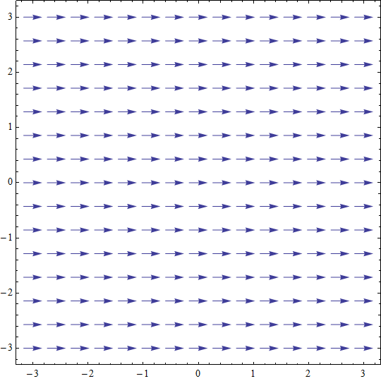
   We therefore add a suitable doublet potential. Its strength is chosen so that the total radial velocity vanishes at:

   $r=R$

   The doublet must exactly cancel the radial component of the uniform flow at the cylinder surface:

   $W=v_{\infty }z=v_{\infty }r{e}^{i\phi }=v_{\infty }r\left(cos\theta +isin\theta \right)$

   $v_r=\frac{\partial }{\partial r}[\mathrm{Re}(W)]=\frac{\partial }{\partial r}(v_{\infty }rcos\theta )=v_{\infty }cos\theta$

   The required potential is that of a two-dimensional doublet (the potential-flow analogue of an electrostatic dipole):

   $\phi =\frac{ccos\theta }{r}$

   $W=\frac{c}{z}$

   The radial component of this field is:

   $v_r=\frac{\partial }{\partial r}[\mathrm{Re}(\phi )]=\frac{\partial }{\partial r}\left(\frac{ccos\theta }{r}\right)=-\frac{ccos\theta }{r^2}$

   At the cylinder surface, the radial components must cancel exactly:

   ${-\frac{ccos\theta }{r^2}|}_{r=R}={-v_{\infty }cos\theta |}_{r=R}$

   $\frac{ccos\theta }{R^2}=v_{\infty }cos\theta$

   $c=v_{\infty }{R}^2$

   $W=\frac{v_{\infty }{R}^2}{z}$

   

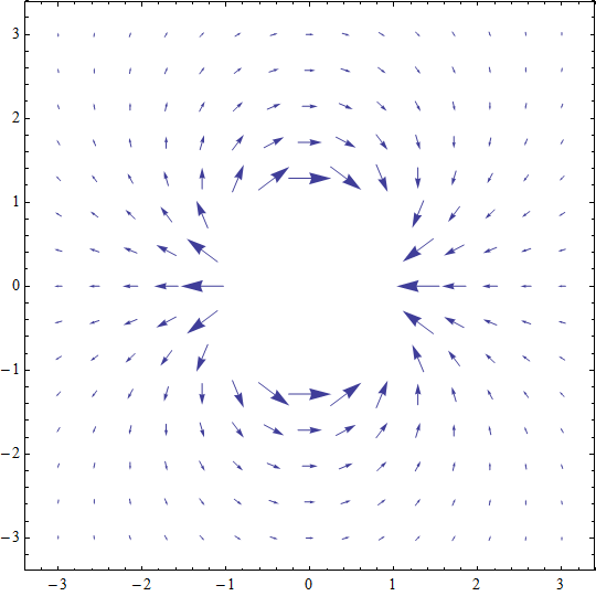
   The resulting combined potential describes inviscid, incompressible, irrotational flow around an impermeable cylinder:

   $W=v_{\infty }z+\frac{v_{\infty }{R}^2}{z}$

   

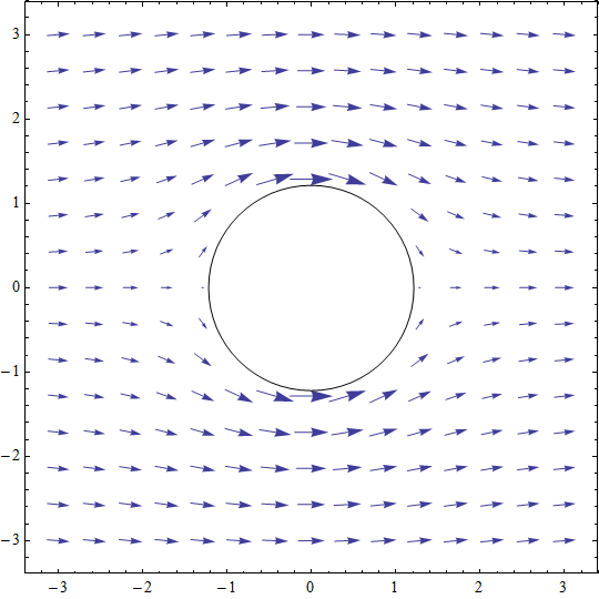
   The velocity field can then be obtained from the potential, and Bernoulli's equation gives the pressure distribution on the surface.

   The resulting pressure is symmetric about the horizontal axis. Consequently, the pressure forces cancel in the vertical direction, and they also cancel in the direction of the freestream.

   The ideal flow predicts:

   $L\prime =0$

   $D\prime =0$

   The prediction of zero drag is the famous d'Alembert paradox.

   A real cylinder clearly experiences drag. The paradox arises because the idealized inviscid flow has eliminated the viscous boundary layer and wake responsible for the real drag.

   But something even more interesting happens when we add circulation.

8. Adding a vortex: the Magnus effect

   A two-dimensional point vortex produces a velocity field:

   $v_r=0$

   $v_{\theta }=-\frac{\Gamma }{2\pi r}$

   Cartesian components of this velocity field are (various equivalent forms):

   $v_x=\frac{\Gamma }{2\pi }\frac{y}{x^2+y^2}=\frac{\Gamma }{2\pi }\frac{y}{r^2}=\frac{\Gamma }{2\pi }\frac{sin\theta }{r}$

   $v_y=-\frac{\Gamma }{2\pi }\frac{x}{x^2+y^2}=-\frac{\Gamma }{2\pi }\frac{x}{r^2}=-\frac{\Gamma }{2\pi }\frac{cos\theta }{r}$

   As expected, the velocity field has zero curl everywhere away from the origin, where the velocity field is singular. In a distributional description, the vorticity is concentrated at the origin:

   $\frac{\partial v_x}{\partial y}-\frac{\partial v_y}{\partial x}=\frac{\Gamma }{2\pi }\frac{x^2-y^2}{{(x^2+y^2)}^2}-\frac{\Gamma }{2\pi }\frac{x^2-y^2}{{(x^2+y^2)}^2}=0$

   The complex potential for this field is:

   $\frac{dW}{dz}=v_x-i{v}_y=\frac{\Gamma }{2\pi }\frac{sin\theta }{r}-i(-\frac{\Gamma }{2\pi }\frac{cos\theta }{r})=\frac{\Gamma }{2\pi }\frac{sin\theta }{r}+i\frac{\Gamma }{2\pi }\frac{cos\theta }{r}=\frac{\Gamma }{2\pi }\frac{sin\theta +icos\theta }{r}=\frac{\Gamma }{2\pi }\frac{i(-isin\theta +cos\theta )}{r}=\frac{\Gamma }{2\pi }\frac{i(cos\theta -isin\theta )}{r}=\frac{\Gamma }{2\pi }\frac{i{e}^{-i\theta }}{r}=\frac{\Gamma }{2\pi }\frac{i}{r{e}^{i\theta }}=\frac{i\Gamma }{2\pi z}$

   $W=\int \frac{i\Gamma }{2\pi z}dz=\frac{i\Gamma lnz}{2\pi }$

   

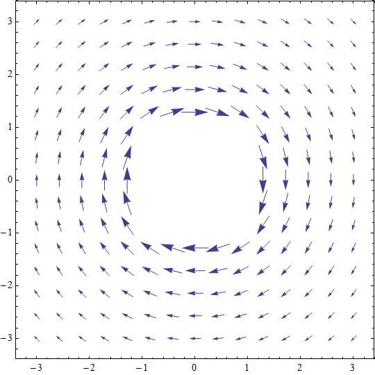
   For this field, velocity is purely tangential, so adding such a vortex to the cylinder flow does not violate the impermeability condition at the cylinder surface.

   The velocity on the upper and lower sides of the cylinder therefore changes by different amounts. On one side, the vortex velocity adds to the freestream-induced velocity; on the other side, it subtracts from it. Combined potential, horizontal flow + doublet + vortex is:

   $W=v_{\infty }z+\frac{v_{\infty }{R}^2}{z}+\frac{i\Gamma lnz}{2\pi }$

   

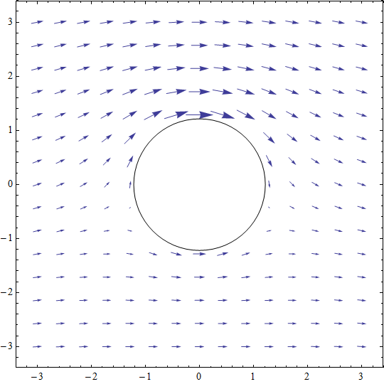
   The entire flow can now be rotated. Geometrically, this changes the direction of the freestream relative to the cylinder. Introducing the rotation at this stage is convenient because it simplifies the subsequent conformal transformation while allowing the angle of attack to be varied. To rotate the flow, we rotate the argument of the potential by multiplying it by a complex exponential. The logarithm changes only by an additive constant, which can be discarded because the velocity depends only on its derivative:

   $W=v_{\infty }z{e}^{-i\alpha }+\frac{v_{\infty }{R}^2}{z{e}^{-i\alpha }}+\frac{i\Gamma lnz}{2\pi }=v_{\infty }z{e}^{-i\alpha }+\frac{v_{\infty }{R}^2}{z}{e}^{i\alpha }+\frac{i\Gamma lnz}{2\pi }$

   

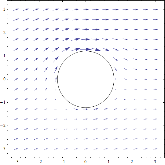
   The pressure distribution becomes asymmetric because the circulation increases the speed on one side of the cylinder and decreases it on the other.

   Integrating the resulting pressure around the cylinder (not evaluated in this article) gives a net transverse force:

   $L\prime =\rho v\Gamma$

   with the sign depending on the convention used for $\Gamma$ (in this article, we consistently use positive value for clockwise circulation).

   This is the Magnus effect.

   The important point is that the Kutta–Joukowski lift relation has appeared naturally from the pressure field of a circulating flow.

   The cylinder is therefore an ideal laboratory for understanding the essential connection:

   circulation → asymmetric velocity → asymmetric pressure → lift

   The remaining problem is to replace the cylinder by an airfoil.

9. Conformal transformations

   Finding potential flow around an arbitrary airfoil is much more difficult than finding the flow around a circle.

   But there is a remarkable property of two-dimensional potential flow: conformal transformations can map one geometry into another while preserving the local structure of the potential-flow solution.

   The most famous example is the Joukowski transformation,

   $z=\zeta +\frac{c^2}{\zeta }$

   Here $\zeta$ represents a point in an auxiliary complex plane containing a circle, while $z$ represents the corresponding point in the physical plane.

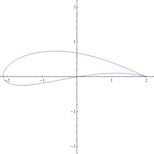
   A suitable circle in the $\zeta$-plane is mapped into an airfoil-like shape in the $z$-plane.

   The circle solution can therefore be transformed into a solution around the resulting airfoil.

   This is the central mathematical idea behind the classical Joukowski airfoil.

   Instead of solving Laplace's equation directly around a complicated wing shape, we solve it around a circle, where the solution is simple, and then transform the solution. Because conformal mappings preserve angles and analytic structure, a potential-flow solution around the circle can be transformed into a potential-flow solution around the mapped airfoil.

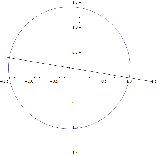
   We apply the transformation to a circle whose center is displaced from the origin in both the horizontal and vertical directions and whose radius is not unity.

   In the following charts, we use these constants:

   $\{\begin{array}{c}{x}_0=\mathrm{-0.2}\\ y_0=0.2\\ c=1\\ \alpha =0.2\text{rad}\end{array}$

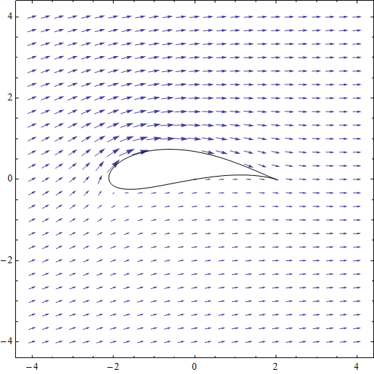
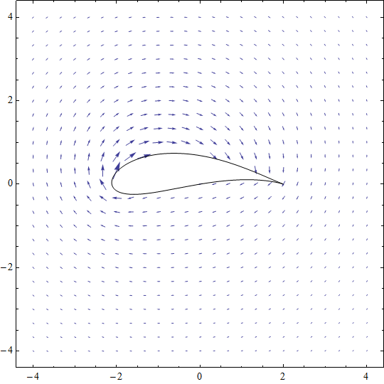
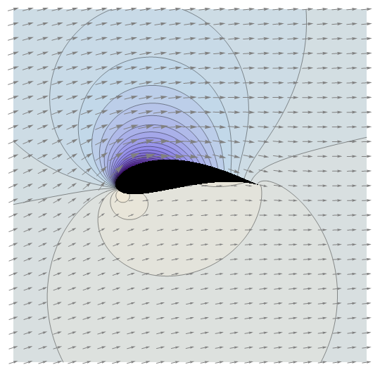
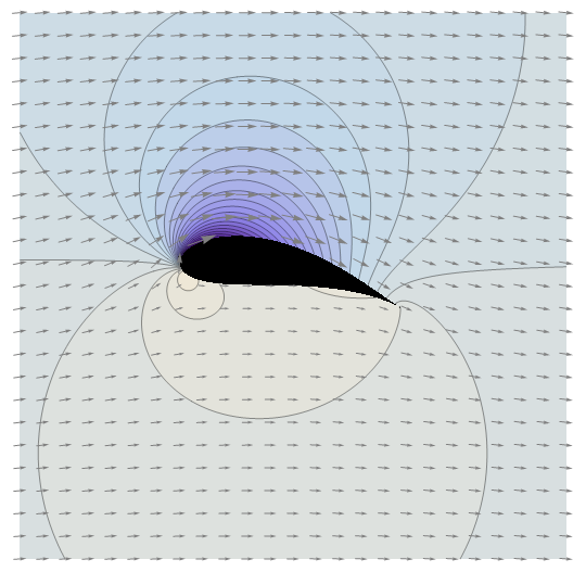
   The center of the original cylinder is located at: $\left(x_0,y_0\right)$. In the following sections, on the left charts, freestream velocity is inclined by angle $\alpha$; on the right charts freestream velocity is horizontal while the airfoil is rotated by angle $\alpha$ instead. Since our ultimate goal is to calculate circulation and lift, we do not need to rotate the frame back so that the freestream velocity is horizontal. For the lift calculation, however, we must use the lift direction perpendicular to the freestream rather than simply the vertical direction. The back-rotation is used only for visualization. Rotating the potential back is trivial: the complex variable is multiplied by the inverse exponential. Angle $\beta$ in later equations is the angle between horizontal axis and line connecting center of the circle with the point on the circle that gets transformed into the cusp. It is defined as a signed angle, measured counterclockwise from the positive horizontal axis. Therefore, it is negative when the line slopes downward, as in the geometry shown in the charts.

   Original cylinder	Joukowski transformation of the cylinder

10. The Joukowski airfoil and circulation

    The complex potential for the cylinder can contain three basic components:

    $W=W_{\text{uniform}}+W_{\text{doublet}}+W_{\text{vortex}}$

    $W=v_{\infty }\zeta e^{-i\alpha }+\frac{v_{\infty }{R}^2}{\zeta }{e}^{i\alpha }+\frac{i\Gamma ln\zeta }{2\pi }$

    The first two create the non-circulating flow around the cylinder. The third introduces an arbitrary circulation $\Gamma$.

    After applying the Joukowski transformation, this becomes a potential flow around an airfoil. As already stated, because of the form of the Joukowski transformation, analysis is easier with inclined freestream velocity, although this is less convenient for visualization; the final plots can be rotated back easily.

    Angle of attack causes freestream velocity to be inclined. This is the plot for velocity obtained from equation above.	Picture rotated back, freestream velocity is horizontal again.

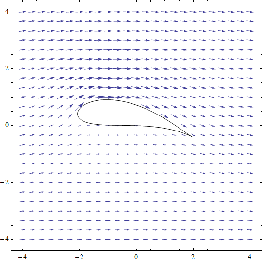    These charts are shown in a frame of reference attached to the moving airfoil. The freestream velocity approaches its constant freestream value at infinite distance. The velocity field therefore appears to pass through the stationary airfoil, but this is only an artifact of the chosen frame: the airfoil is moving through the air, and the fluid occupies the space vacated by the airfoil.

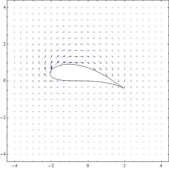    At this stage, however, $\Gamma$ is still arbitrary.

    This is where the Kutta condition returns.

    The trailing edge of a Joukowski airfoil corresponds to a special point of the transformation. At this point, the derivative of the transformation vanishes:

    $\frac{dz}{d\zeta }=\frac{d}{d\zeta }(\zeta +\frac{c^2}{\zeta })=1-\frac{c^2}{{\zeta }^2}$

    ${\frac{dz}{d\zeta }|}_{\zeta =c}={[1-\frac{c^2}{{\zeta }^2}]}_{\zeta =c}=0$

    Because the physical velocity involves the transformation of the complex velocity, an inappropriate choice of circulation can cause the velocity at the trailing edge to become infinite.

    As noted above, the circle that we want to transform is neither centered at the origin nor of unit radius. The center of the circle is displaced from the origin by:

    ${\zeta }_0=x_0+y_{0}i$

    The circle must also pass through the special point of the transformation to get a cusp in the back of the profile. This determines the radius:

    $R=|c-{\zeta }_0|$

    Because the center has been translated, the potential must be modified by the same translation:

    $W=v_{\infty }(\zeta -{\zeta }_0)e^{-i\alpha }+\frac{v_{\infty }{R}^2}{\zeta -{\zeta }_0}{e}^{i\alpha }+\frac{i\Gamma ln(\zeta -{\zeta }_0)}{2\pi }$

    Complexified velocity field for the new potential is:

    $\frac{dW}{d\zeta }=v_{\infty }{e}^{-i\alpha }-\frac{v_{\infty }{R}^2}{{(\zeta -{\zeta }_0)}^2}{e}^{i\alpha }+\frac{i\Gamma }{2\pi (\zeta -{\zeta }_0)}$

    The velocity in the physical airfoil plane is obtained by the chain rule:

    $\frac{dW}{dz}=\frac{dW}{d\zeta }\frac{d\zeta }{dz}=\frac{dW}{d\zeta }\frac{1}{\frac{dz}{d\zeta }}$

    At the trailing edge $\zeta =c$, both the numerator and denominator of this transformed velocity must vanish to avoid a singularity. The calculation below therefore imposes:

    ${\frac{dW}{d\zeta }|}_{\zeta =c}=0$

    Which is the Kutta condition in this construction.

    The behavior near the cusp is:

    ${\frac{dW}{d\zeta }|}_{\zeta =c}=v_{\infty }{e}^{-i\alpha }-\frac{v_{\infty }{|c-{\zeta }_0|}^2}{{(c-{\zeta }_0)}^2}{e}^{i\alpha }+\frac{i\Gamma }{2\pi (c-{\zeta }_0)}$

    We can rewrite the denominator of the second term and third term to absolute value + exponent form to simplify the fraction:

    ${\frac{dW}{d\zeta }|}_{\zeta =c}=v_{\infty }{e}^{-i\alpha }-\frac{v_{\infty }{|c-{\zeta }_0|}^2}{{|c-{\zeta }_0|}^2{e}^{2i\beta }}{e}^{i\alpha }+\frac{i\Gamma }{2\pi |c-{\zeta }_0|e^{i\beta }}$

    ${\frac{dW}{d\zeta }|}_{\zeta =c}=v_{\infty }{e}^{-i\alpha }-\frac{v_{\infty }}{e^{2i\beta }}{e}^{i\alpha }+\frac{i\Gamma }{2\pi R{e}^{i\beta }}$

    ${\frac{dW}{d\zeta }|}_{\zeta =c}=v_{\infty }{e}^{-i\alpha }-v_{\infty }{e}^{-2i\beta }{e}^{i\alpha }+\frac{i\Gamma }{2\pi R}{e}^{-i\beta }$

    Where $\beta$ is the angle (complex argument):

    $\beta =-arctan\frac{y_0}{c-x_0}=-arcsin\frac{y_0}{R}$

    We must choose the circulation so that the numerator vanishes at the cusp, cancelling the singular behavior produced by the vanishing derivative of the conformal map:

    $v_{\infty }{e}^{-i\alpha }-v_{\infty }{e}^{-2i\beta }{e}^{i\alpha }+\frac{i\Gamma }{2\pi R}{e}^{-i\beta }=0$

    $-\frac{i\Gamma }{2\pi R}{e}^{-i\beta }=v_{\infty }{e}^{-i\alpha }-v_{\infty }{e}^{-2i\beta }{e}^{i\alpha }$

    $\Gamma =2\pi Ri{e}^{i\beta }{v}_{\infty }(e^{-i\alpha }-e^{-2i\beta }{e}^{i\alpha })=2\pi Ri{v}_{\infty }(e^{-i\alpha }{e}^{i\beta }-e^{-i\beta }{e}^{i\alpha })=2\pi Ri{v}_{\infty }(e^{i(-\alpha +\beta )}-e^{-i(-\alpha +\beta )})=-4\pi R{v}_{\infty }sin(-\alpha +\beta )=4\pi R{v}_{\infty }sin(\alpha -\beta )=4\pi R{v}_{\infty }sin(\alpha +arcsin\frac{y_0}{R})$

    The Kutta condition determines the unique circulation for which the trailing-edge singularity is removed and the flow leaves the trailing edge smoothly.

    Thus the Kutta condition determines:

    $\Gamma =4\pi R{v}_{\infty }sin(\alpha -\beta )=4\pi R{v}_{\infty }sin(\alpha +arcsin\frac{y_0}{R})$

    Once this value is known, the Kutta–Joukowski theorem immediately gives the lift.

    The entire calculation has therefore reduced to finding the circulation required by the Kutta condition.

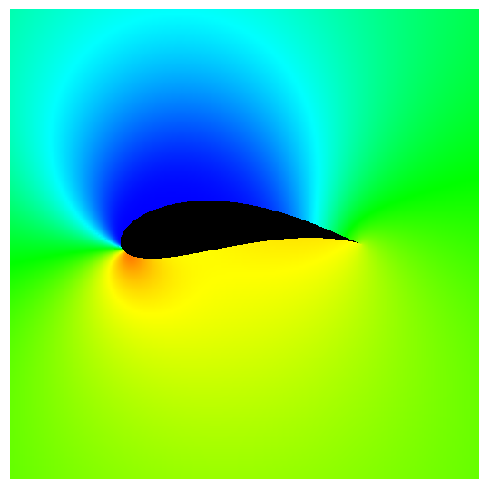
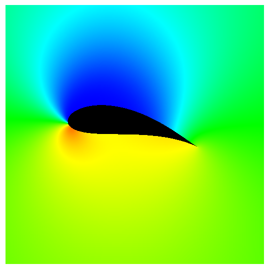
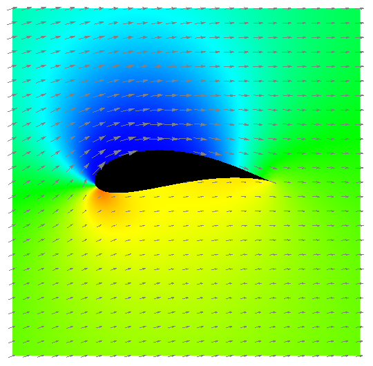
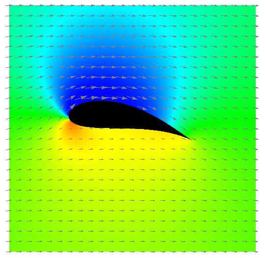
    The following plots show the pressure and velocity fields. The first row shows the pressure field (red/orange indicates high pressure and blue indicates low pressure); the second row shows the pressure field with the velocity field superimposed; and the third row shows isobars with the velocity field superimposed. The left images use the coordinates convenient for the calculation, with the freestream velocity inclined. The right images are rotated back to the natural visualization orientation, with the freestream velocity horizontal.

11. What the classical solution teaches us

    The Joukowski construction is more than an elegant historical solution to an aerodynamic problem. It illustrates the structure of aerodynamic lift remarkably well.

    At the most fundamental level, the fluid obeys conservation laws; constitutive relations then close the equations and, for a Newtonian fluid, lead to the Navier–Stokes equations.

    For a real aircraft, those equations must account for viscosity, boundary layers, turbulence, separation, compressibility, and the three-dimensional geometry of the aircraft. Exact analytical solutions are generally impossible.

    Nevertheless, by considering a simplified regime:

    incompressible + inviscid + irrotational

    the problem becomes:

    $∆\phi =0$

    In two dimensions, complex analysis provides a powerful way to construct solutions of this equation. The flow around a cylinder can be built from elementary potentials, and circulation can be added independently.

    The resulting circulating flow produces an asymmetric pressure distribution and hence lift.

    A conformal transformation then converts the cylinder into an airfoil.

    Finally, the Kutta condition selects the physically relevant circulation.

    The logical chain is therefore:

    Conservation laws → Navier–Stokes equations → idealized potential flow → Laplace equation → complex potential → cylinder + circulation → Magnus effect → Joukowski transformation → airfoil → Kutta condition → lift

    There is also a particularly interesting conceptual lesson hidden in this derivation. The mathematical model used to calculate the lift is inviscid, yet the selection of the circulation is fundamentally connected with viscous effects at the trailing edge and in the wake. Thus the classical theory does not simply say that viscosity is irrelevant. Rather, it separates the problem into two roles: the inviscid flow determines how a given circulation produces lift, while the physics of the real flow determines which circulation occurs.

    That is why the apparently simple formula:

    $L\prime =\rho v\Gamma$

    contains considerably more physics than its short form suggests.